Realistic Looking and Optimal A* Path Planning: Theta*

1. Introduction

Finding short and realistic looking paths is the challengeable topic to attract most game developers and roboticists. There are several reasons why they focus on it: realistic paths make game players concentrate on a game more efficiently and make game characters intelligent and robots can save energy by choosing a shortest path. As a result, diverse algorithms have been introduced such as A*, visibility graph, RRT, and so on. One of the most popular and optimal algorithm is A* because A* is guaranteed to find a shortest path on the graph. However, a shortest path as result of A* is unrealistic and longer in the continuous environment. To solve the problem, a post processing technique to make a path smooth and short is applied in general but original A* doesn’t consider path smoothing in finding a shortest path. Thus, there is possibility that the post processed results cannot be the optimal path. Our solution in this project is to apply the visibility graph algorithm, Theta*[1] in calculating heuristic. The main difference between Theta* and A* is to check the visibility between the neighbor of a current vertex and the parent of current vertex. If visibility is true and the cost of two vertices is less than the cost of via current vertex, the parent vertex of the neighbor vertex is the parent of the current vertex. Consequently, Theta* can find shorter and more realistic path than A* and post processed A*.

2. Related Work

Path shortening and smoothing in grid-based A*[2] is the post processed results, thus it can make a path realistic. On the other hand, it cannot find a more optimal path, since A* search can find one of shortest paths on the graph using a certain heuristic, but others can be smoothed or shorten more effectively than the result. Visibility graph[3] has pairs of points are connected by an edge if they can be joined by a straight line without intersecting any obstacles. It is doomed to have at least quadratic running time in the worst case. Therefore, it is necessary to consider how to overcome this problem in Theta* also.

3. Notation

S is the set of all grid vertices, s_start ∈ S is the start vertex of the search, and s_goal ∈ S is the goal vertex of the search. succ(s) ⊆ S is the set of neighbors of s ∈ S that have line-of-sight to s. c(s, s′) is the straight-line distance between s and s′ (both not necessarily vertices), and Lineofsight(s, s′) is true if and only if they have line-of-sight.

4. Approach

The key difference between Theta* and A* is that Theta* allows the parent of a vertex to be any vertex, unlike A* where the parent must be a visible neighbor. Theta* is identical to A* except that Theta* updates the g-value and parent of an unexpanded visible neighbor s’ of vertex s as Algorithm 1 describes.

Algorithm 1. Pseudo Code for Calculating Cost in Theta*

As done by A*, Theta* considers the path from the start vertex to s [= g(s)] and from s to s’ in a straight line [= c(s,s')], resulting in a length of g(s) + c(s,s’) (Line 9 in Algorithm 1). To allow for any-angle paths, Theta* also considers the path from the start vertex to parent(s) [= g(parent(s))] and from parent(s) to s’ in a straight line [= c(parent(s),s')], resulting in a length of g(parent(s)) + c(parent(s),s’) if s’ has line-of-sight to parent(s) (Line 4 in Algorithm 1). The idea behind considering Path 2 is that Path 2 is no longer than Path 1 due to the triangle inequality if s’ has Lineofsight to parent(s). Theta* performs its Line-of-sight checks with a standard line-drawing method from computer graphics[5] that uses only fast logical and integer operations rather than floating-point operations.

A* and Theta* are implemented as a class and A* PS shortens a result of A*. A* PS runs A* on grids and then shortens the resulting path in a post-processing step. Algorithm 2 shows the pseudocode of the simple smoothing algorithm that A* PS uses in this paper.

Algorithm 2. Pseudo Code for A* Post Smooth

Figure 1. Completeness Test in various maps

Figure 2. Paths found by A*, A* PS, and Theta* in a polygon map, (a)A*, Tile (b)A* PS, Tile (c)Theta*, Tile (d)A*, Octile (e)A* PS, Octile (f)Theta*, Octile

5. Evaluation

All algorithms are run on dual-core 2.66 GHz, 4GB RAM, and Window 7 64-bit. The width of the map is 157 and the height of the map is 169. We evaluate completeness, optimality and efficiency of A*, A* PS, and Theta* in different grid map structures: tile and octile. First, to test completeness, we made maps which haven’t a path to a goal. A*, A* PS and Theta* are evaluated on the maps and Figure 1 depicts that A*, A* PS and Theta* show the message when there are no node to explore.

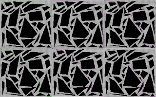
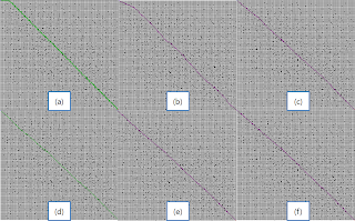
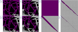
Optimality and efficiency are tested with A*, A* PS and Theta* on a map which Figure 2 and Figure 3 illustrate. To compare optimality each algorithm, we calculate distance from a start point to a goal. We measure the elapsed time to search a path from a start point to a goal point for efficiency. Additionally, nodes which examined during searching in A* and Theta* are displayed and counted in Figure 4 in order to analyze which factor affects the efficiency. We don’t include examined nodes of A* PS because A* PS elaborates a path based on the result of A*.

Figure 3. Paths found by A*, A* PS, and Theta* in a random map (a)A*, Tile (b)A* PS, Tile (c)Theta*, Tile (d)A*, Octile (e)A* PS, Octile (f)Theta*, Octile

Figure 4. Examined nodes in a polygon map and a random map (a)A* and A* PS Tile (b)Theta*, Tile (c)A* and A* PS, Octile (d) Theta*, Octile

6. Discussion

Figure 2 and Table 1 exhibit that Theta* is the most efficient algorithm in a tile map structure. The main reason is that Theta* examined less nodes than A* and A* PS as Figure 4 and Table 1 illustrate. However, Theta* which has even less examined nodes is less efficient than A* and A* PS in octile representation since Theta* executes LineOfSight to expanded nodes, and the LineOfSight is a time consuming process. However, in a random map in Figure 3, Theta* is the most efficient algorithm in both map structures due to the fact that expanded nodes of Theta* is significantly less than A* and A* PS. Since g-values in Theta* is the distance of a straight line from a current node to a start node, we can avoid tie in calculating f-values, and Theta* can search less nodes than other algorithms.

In the perspective view of optimality, Theta* is the most efficient algorithm in both map representations, but the distance difference between Theta* and A* PS is tiny. A* PS has the process to check LineOfSight in order to shorten a result path. Thus, if a result of A* is similar with Theta*, distance to a goal of Theta* and A* PS is almost same, but if the result of A* is different with Theta*, distance to a goal of A* PS is quite different with Theta* as Figure 2 and Table 1 describe.

Table 1. Distance, elapsed time, and examined nodes with A*, A* PS and Theta in a polygon and a random map

	Polygon Map			Random Map
	Cost toGoal	Elapsed Time(msec)	# of Examined Node	Cost toGoal	Elapsed Time(msec)	# of Examined Node
A*Tile	324	30	11107	324	70	25128
A* PSTile	300.4	35	11107	231.472	70	25128
Theta*Tile	267.919	27	6251	229.556	7	1475
A*Octile	276.149	22	7034	232.618	12	2659
A* PSOctile	262.494	22	7034	229.403	12	2659
Theta*Octile	262.352	26	5487	229.383	3	334

Theta* is complete as Figure 1 depicts and is more optimal and efficient than A* and A* PS in a tile map structure, not in an octile representation. A tile map is memory efficient since you can reduce edges for diagonal directions. Thus, if your robot and virtual agent must explore a large map and you have a memory issue, Theta* can find short realistic looking paths efficiently.

In this paper, we evaluate Theta* in tile and octile map structure. Future research will be to support extending Theta* to grids whose cells have non-uniform sizes and traversal costs.

Execution File

7. References

[1] Nash, A., Daniel, K., & Felner, S. K. A. (2007). Theta*: Any-angle path planning on grids. In Proceedings of the National Conference on Artificial Intelligence, pp. 1177–1183

[2] Kanehara, M., Kagami, S., Kuffner, J.J., Thompson, S., Mizoguhi, H. (2007). Path shortening and smoothing of grid-based path planning with consideration of obstacles. Systems, Man and Cybernetics, pp. 991-996

[3] D. Ferguson and A. Stentz. (2006). An Algorithm for Planning Collision-free Paths among Polyhedral Obstacles. Journal of Field Robotics, Volume 23, Issue 2, pp. 79-101

[4] Y. Bjornsson, M. Enzenberger, R. Holte, J. Schaeffer and P. Yap. (2003). Comparison of Different Grid Abstractions for Pathfinding on Maps. Proceedings of the International Joint Conference on Artificial Intelligence, pp. 1511-1512

[5] J. Bresenham. (1965). IBM Systems Journal, Volume 4, Issue 1, pp. 25-30

Machine Learning Algorithms

1. Q-learning

Path Planning Algorithms

What is Q-learning and How to implement a resuable Q-learning?

1. Introduction

You may have a difficulty in making your software to be adaptable on interaction with human. The main reason is that in general, it is very hard to expect people’s responses in previous at various situations. How to solve the problem? If a machine can change its internal parameters based on a uses’ intention, an adaptable system can be built. One of solutions is a machine learning algorithm and Q-learning can be used. Since it is reinforcement learning, a system can adapt or change itself based on interactions with human. In this lecture, I will address the theory of Q-learning, software architecture of the machine learning, and examples.

2. Theory

Machine learning algorithms can be divided into several categories by learning method: supervised learning, reinforcement learning, unsupervised learning, etc. In case of Q-learning, it is reinforcement learning, because it receives feedback to guide the learning algorithm from environment and acts. In 1989, Watkins introduced it and it is used in numerous areas such as robotics, game, industry and so on. The reasons which let the learning algorithm widespread are that the algorithm is very simple and easy to implement and shows good result in some applications. However, it has also flaws: If states and actions are so big, the performance gets bad. It will not try for better actions in a particular state and will repeat one action when it takes an action to show good results.

Let's take a look at the algorithm of Q-learning, Aforementioned, Q-learning is composed with actions, states, rewards, Q-values and parameters. Their definitions are:

• An action is to change a state to another state.
• A state is to describe a certain situation.
• A Reward is a feedback from doing an action in a state.
• Q-value is a value used in choosing an action from numerous actions in a state.

Q-values that are the result of Q-learning are obtained by learning process described in Equation-1. The core of the algorithm is to update the Q-values based on new rewards.

Equation-1

2. Implementation

In this chapter, I will describe how to implement reusable Q-learning with C++. To implement a reusable Q-learning, I design the software architecture of Q-learning that separates the core algorithm and configurable parts. If you mix them, you have to make a new Q-learning for every applications. Fig.1 shows Q-learning class diagram and it is composed with state, action, and Q-learning class. The state class contains all variables to compose a state and has all related actions. The action class has reward and Q-value which are updated by Q-learning algorithm. The Q-learning class manages all state and actions and updates Q-values. The configurable parts are states and actions, because they are defined differently by problems. Therefore, I placed all information about states and actions in a XML file in order to avoid changing the core source code of Q-learning. Unfortunately, making a configuration file is an onerous job, because there will be tens or hundreds of actions and states for solving just one problem. Therefore, I made a GUI to make configuration files with ease. Using this GUI, you can define states and actions which will be used on various problems and create a XML file to contain all information about Q-learning and can be imported to the core source code of Q-learning.

Fig.1 Class Diagram of Q-learning

Fig.2 Graphical User Interface for Q-learning

Understanding a variety of algorithms and apply them to certain problems appropriately are very important, but making reusable software of algorithms is crucial, too. If you don’t make reusable software programs, you spend enormous time to make software programs to work out each problem. At first, when you try to make a reusable software program, you may feel that it is useless and it is waste of time. However, whenever you confront a situation to solve a problem with a previous software program of the same algorithm, you would think that I should have made a reusable one. Consequently, if you design a software program, you should spend enough time to design it as reusable one. If you do that, I strongly believe that you would save our time magnificently later.

Video Clip to Show Solving Tower of Hanoi